How I Built This
Caveat: this is my first ever attempt at building a linear regression model end to end. It's basic, but a good learning exercise!
Gather training data
I collected some data with a simple scrape of Immobilien Scout, scraping 252 samples. Number of rooms, and square metres of floor space were the two features I selected, whilst the listing price was the label.
import numpy as np

x_train = np.array([
    [
        4,
        152
    ],
    [
        3,
        66
    ],
    # ...
)
import numpy as np

y_train = np.array([
    1550000,
    499000,
    # ...
    )
Run gradient descent to calculate model weights
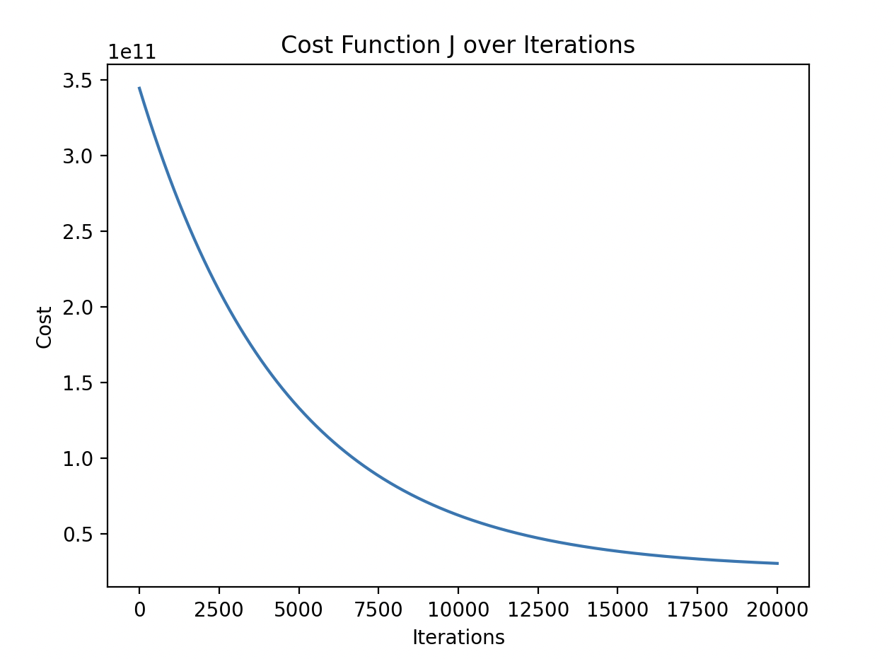
I then ran a standard gradient descent model on the data. It took some tweaks to the iteration count, learning rate and initial parameters to get the model to converge.
import numpy as np

# Training data
from x import x_train

# Training Labels
from y import y_train

# Functions
from functions import compute_cost, compute_gradient, gradient_descent

# initialize parameters
initial_w = np.array([0.75376741, 0.00039133535])
initial_b = 0

# some gradient descent settings
iterations = 20000
alpha = 1.0e-8

# run gradient descent
w_final, b_final, J_hist = gradient_descent(
    x_train, y_train, initial_w, initial_b, compute_cost, compute_gradient, alpha, iterations)
import copy
import numpy as np
import math
from y import y_train

def gradient_descent(X, y, w_in, b_in, cost_function, gradient_function, alpha, num_iters):
    """
    Performs batch gradient descent to learn w and b. Updates w and b by taking
    num_iters gradient steps with learning rate alpha

    Args:
      X (ndarray (m,n))   : Data, m examples with n features
      y (ndarray (m,))    : target values
      w_in (ndarray (n,)) : initial model parameters
      b_in (scalar)       : initial model parameter
      cost_function       : function to compute cost
      gradient_function   : function to compute the gradient
      alpha (float)       : Learning rate
      num_iters (int)     : number of iterations to run gradient descent

    Returns:
      w (ndarray (n,)) : Updated values of parameters
      b (scalar)       : Updated value of parameter
      """

    # An array to store cost J and w's at each iteration primarily for graphing later
    J_history = []
    w = copy.deepcopy(w_in)  # avoid modifying global w within function
    b = b_in

    for i in range(num_iters):

        # Calculate the gradient and update the parameters
        dj_db, dj_dw = gradient_function(X, y, w, b)  # None

        # Update Parameters using w, b, alpha and gradient
        w = w - alpha * dj_dw  # None
        b = b - alpha * dj_db  # None

        # Save cost J at each iteration
        if i < 100000:      # prevent resource exhaustion
            J_history.append(cost_function(X, y, w, b))

        # Print cost every at intervals 10 times or as many iterations if < 10
        # if i % math.ceil(num_iters / 10) == 0:
        #     print(f"Iteration {i:4d}: Cost {J_history[-1]:8.2f}   ")

    return w, b, J_history  # return final w,b and J history for graphing


def compute_cost(X, y, w, b):
    """
    compute cost
    Args:
      X (ndarray (m,n)): Data, m examples with n features
      y (ndarray (m,)) : target values
      w (ndarray (n,)) : model parameters
      b (scalar)       : model parameter

    Returns:
      cost (scalar): cost
    """
    m = X.shape[0]
    cost = 0.0
    for i in range(m):
        f_wb_i = np.dot(X[i], w) + b  # (n,)(n,) = scalar (see np.dot)
        cost = cost + (f_wb_i - y[i])**2  # scalar
    cost = cost / (2 * m)  # scalar
    return cost


def compute_gradient(X, y, w, b):
    """
    Computes the gradient for linear regression
    Args:
      X (ndarray (m,n)): Data, m examples with n features
      y (ndarray (m,)) : target values
      w (ndarray (n,)) : model parameters
      b (scalar)       : model parameter

    Returns:
      dj_dw (ndarray (n,)): The gradient of the cost w.r.t. the parameters w.
      dj_db (scalar):       The gradient of the cost w.r.t. the parameter b.
    """
    m, n = X.shape  # (number of examples, number of features)
    dj_dw = np.zeros((n,))
    dj_db = 0.

    for i in range(m):
        err = (np.dot(X[i], w) + b) - y[i]
        for j in range(n):
            dj_dw[j] = dj_dw[j] + err * X[i, j]
        dj_db = dj_db + err
    dj_dw = dj_dw / m
    dj_db = dj_db / m

    return dj_db, dj_dw
Review Results
The results are in! These are what are used in the model above in the end.
# bias and weights that were found
b,w found by gradient descent: 119.32,[ 201.47428015 6772.49617494]
Evaluate Model
I used a Mean Error Percentage to evaluate the effectiveness/accuracy of the model - basically, on average, how far off was I in my estimated house prices if I used the model on the existing training date
# Mean Error Percentage
predictions = x_train.dot(w_final) + b_final
percentage_errors = 100 * np.abs((predictions - y_train) / y_train)
mean_error_percentage = np.mean(percentage_errors)
print(f"Mean Error Percentage: {mean_error_percentage:0.2f}%")
# mean error percentage is still quite high! I tried feature scaling
# but it didn't help much, I think the data is just too noisy
Mean Error Percentage: 20.90%
Plot Data
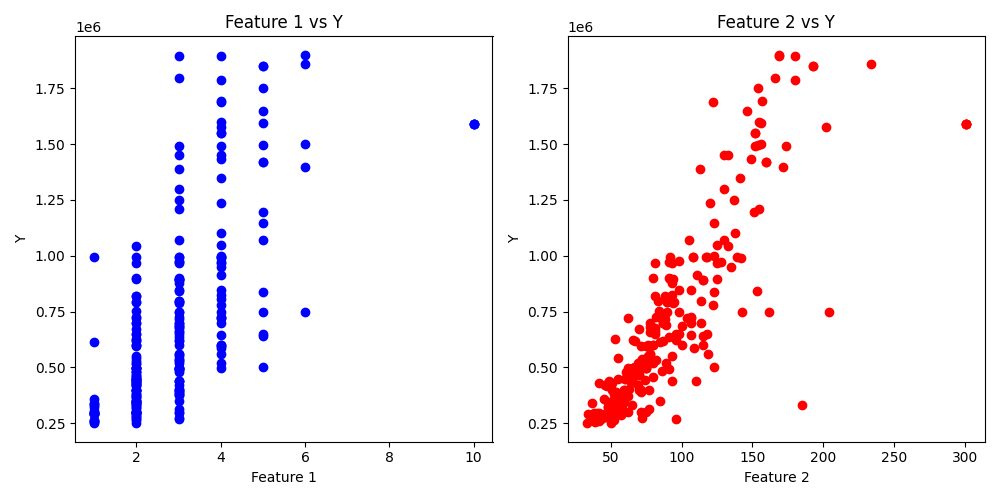
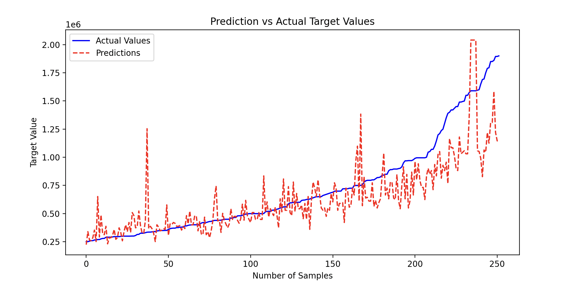
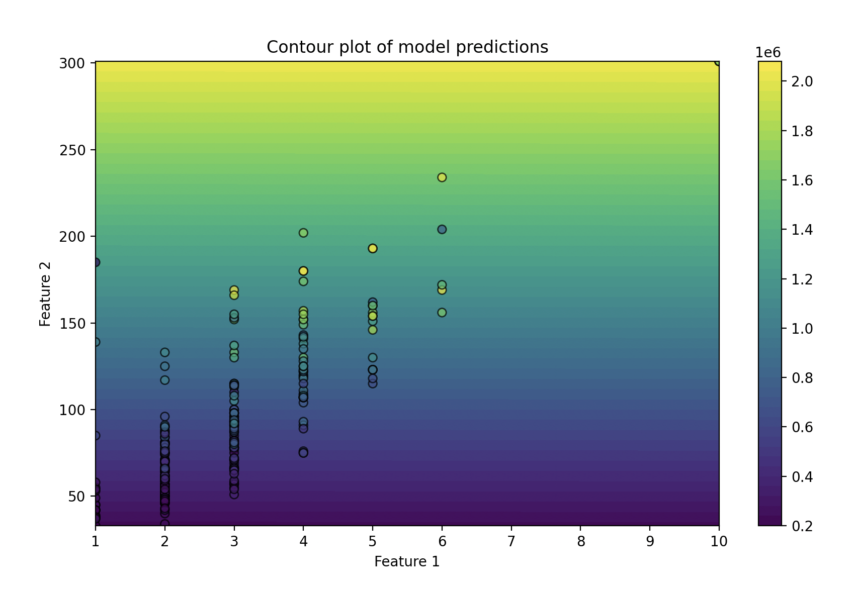
I thought plotting the data might help me visualise how the model could be improved, so I plotted:
- Each feature against the label
- The cost function
- The model's predictions if I used the mean price as the prediction
- A 2D contour plot
Optimize
From the results and plots above I was able to determine that the model isn't as accurate for the top ~20% of house prices. I tried using weighted costs (1.5x for the bottom 80% of data points), but it didn't improve the model.
I also tried Feature Scaling, but did not experience success - it didn't offer better predictions than the original model.
In hindsight, I could have collected more features to play around with and see the relationship. It appears that, from the data collected, that space is far more influential on listing price than the number of rooms.
